

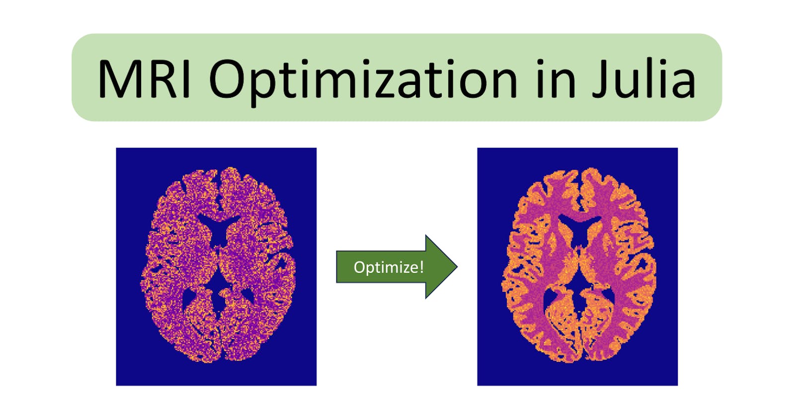
Efficient Julia Optimization through an MRI Case Study
Check out this Julia code example illustrating the optimization of input parameters to reduce a cost function.


Welcome to our first Julia for Devs blog post! This will be a continuously running series of posts where our team will discuss how we have used Julia to solve real-life problems. So, let's get started!
In this Julia for Devs post, we will discuss using Julia to optimize scan parameters in magnetic resonance imaging (MRI).
If you are interested just in seeing example code showing how to use Julia to optimize your own cost function, feel free to skip ahead.
While we will discuss MRI specifically, the concepts (and even some of the code) we will see will be applicable in many situations where optimization is useful, particularly when there is a model for an observable signal. The model could be, e.g., a mathematical equation or a trained neural network, and the observable signal (aka the output of the model) could be, e.g., the image intensity of a medical imaging scan or the energy needed to heat a building.
Problem Setup
In this post, the signal model we will use is a mathematical equation that gives the image intensity of a balanced steady-state free precession (bSSFP) MRI scan. This model has two sets of inputs: those that are user-defined and those that are not. In MRI, user-defined inputs are scan parameters, such as how long to run the scan for or how much power to use to generate MRI signal. The other input parameters are called tissue parameters because they are properties that are intrinsic to the imaged tissue (e.g., muscle, brain, etc.).
Tissue parameters often are assumed to take on a pre-defined value for each specific tissue type. However, because they are tissue-specific and can vary with health and age, sometimes tissue parameters are considered to be unknown values that need to be estimated from data.
The problem we will discuss in this post is how to estimate tissue parameters from a set of bSSFP scans. Then we will discuss how to optimize the scan parameters of the set of bSSFP scans to improve the tissue parameter estimates.
To estimate tissue parameters, we need the following:
- a signal model, and
- an estimation algorithm.
Signal Model
Here's the signal model:
# Reference: https://www.mriquestions.com/true-fispfiesta.html
function bssfp(TR, flip, T1, T2)

    E1 = exp(-TR / T1)
    E2 = exp(-TR / T2)
    (sinα, cosα) = sincosd(flip)
    num = sinα * (1 - E1)
    den = 1 - cosα * (E1 - E2) - E1 * E2
    signal = num / den

    return signal

end
This function returns the bSSFP signal
as a function of two scan parameters
(TR, a value in units of seconds,
and flip, a value in units of degrees)
and two tissue parameters
(T1 and T2, each a value in units of seconds).
Estimation Algorithm
There are various estimation algorithms out there,
but, for simplicity in this post,
we will stick with a grid search.
We will compute the bSSFP signal
over many pairs of T1 and T2 values.
We will compare these computed signals
to the actual observed signal,
and the pair of T1 and T2 values
that results in the closest match
will be chosen as the estimates of the tissue parameters.
Here's the algorithm in code:
# `signal` is the observed signal.
# `TR` and `flip` are the scan parameters that were used,
# and we want to estimate `T1` and `T2`.
# `signal`, `TR` and `flip` should be vectors of the same length,
# representing running multiple scans
# and recording the observed signal for each pair of `TR` and `flip` values.
function gridsearch(signal, TR, flip)

    # Specify the grid of values to search over.
    # `T1_grid` and `T2_grid` could optionally be inputs to this function.
    T1_grid = exp10.(range(log10(0.5), log10(3), 40))
    T2_grid = exp10.(range(log10(0.005), log10(0.7), 40))

    T1_est = T1_grid[1]
    T2_est = T2_grid[1]
    best = Inf
    # Pre-allocate memory for some computations to speed up the following loop.
    residual = similar(signal)
    # Iterate over the Cartesian product of `T1_grid` and `T2_grid`.
    for (T1, T2) in Iterators.product(T1_grid, T2_grid)
        # Physical constraint: T1 is greater than T2, and both are positive.
        T1 > T2 > 0 || continue
        # For the given T1 and T2 pairs, compute the (noiseless) bSSFP signal
        # for each bSSFP scan and subtract them from the given signals.
        # Tip: In Julia, one can apply a scalar function elementwise on vector
        #      inputs using the "dot" notation (see the `.` after `bssfp` below).
        residual .= signal .- bssfp.(TR, flip, T1, T2)
        # Compute the norm squared of the above difference.
        err = residual' * residual
        # If the candidate T1 and T2 pair fit the given signals better,
        # keep them as the current estimate of T1 and T2.
        if err < best
            best = err
            T1_est = T1
            T2_est = T2
        end
    end

    isinf(best) && error("no valid grid points; consider changing `T1_grid` and/or `T2_grid`")

    return (T1_est, T2_est)

end
Cost Function
Now, to optimize scan parameters we need a function to optimize, also called a cost function. In this case, we want to minimize the error between what our estimator tells us and the true tissue parameter values. But because we need to optimize scan parameters before running any scans, we will simulate bSSFP MRI scans using the given sets of scan parameters and average the estimator error over several sets of tissue parameters. Here's the code for the cost function:
# Load the Statistics standard library package to get access to the `mean` function.
using Statistics

# `TR` and `flip` are vectors of the same length
# specifying the pairs of scan parameters to use.
function estimator_error(TR, flip)

    # Specify the grid of values to average over and the noise level to simulate.
    # For a given pair of `T1_true` and `T2_true` values,
    # bSSFP signals will be simulated, and then the estimator
    # will attempt to estimate what `T1_true` and `T2_true` values were used
    # based on the simulated bSSFP signals and the given scan parameters.
    T1_true = [0.8, 1.0, 1.5]
    T2_true = [0.05, 0.08, 0.1]
    noise_level = 0.01

    T1_avg = mean(T1_true)
    T2_avg = mean(T2_true)
    # Pre-allocate memory for some computations to speed up the following loop.
    signal = float.(TR)
    # The following computes the mean estimator error over all pairs
    # of true T1 and T2 values.
    return mean(Iterators.product(T1_true, T2_true)) do (T1, T2)
        # Ignore pairs for which `T2 > T1`.
        T2 > T1 && return 0
        # Simulate noisy signal using the true T1 and T2 values.
        signal .= bssfp.(TR, flip, T1, T2) .+ noise_level .* randn.()
        # Estimate T1 and T2 from the noisy signal.
        (T1_est, T2_est) = gridsearch(signal, TR, flip)
        # Compare estimates to truth.
        T1_err = (T1_est - T1)^2
        T2_err = (T2_est - T2)^2
        # Combine the T1 and T2 errors into one single error metric
        # by averaging the respective errors
        # after normalizing by the mean true value of each parameter.
        err = (T1_err / T1_avg + T2_err / T2_avg) / 2
    end

end
Optimization
Now we are finally ready to optimize! We will use Optimization.jl. Many optimizers are available, but because we have a non-convex optimization problem, we will use the adaptive particle swarm global optimization algorithm. Here's a function that does the optimization:
# Load needed packages.
# Optimization.jl provides the optimization infrastructure,
# while OptimizationOptimJL.jl wraps the Optim.jl package
# that provides the optimization algorithm we will use.
using Optimization, OptimizationOptimJL

# Load the Random standard library package to enable setting the random seed.
using Random

# `TR_init` and `flip_init` are vectors of the same length
# that provide a starting point for the optimization algorithm.
# The length of these vectors also determines the number of bSSFP scans to simulate.
function scan_optimization(TR_init, flip_init)

    # Ensure randomly generated noise is the same for each evaluation.
    Random.seed!(0)

    N_scans = length(TR_init)
    length(flip_init) == N_scans || error("`TR_init` and `flip_init` have different lengths")

    # The following converts the cost function we created (`estimator_error`)
    # into a form that Optimization.jl can use.
    # Specifically, Optimization.jl needs a cost function that takes two inputs
    # (the first of which contains the parameters to optimize)
    # and returns a real number.
    # The input `x` is a concatenation of `TR` and `flip`,
    # i.e., `TR == x[1:N_scans]` and `flip == x[N_scans+1:end]`.
    # The input `p` is unused, but is needed by Optimization.jl.
    cost_fun = (x, p) -> estimator_error(x[1:N_scans], x[N_scans+1:end])

    # Specify constraints.
    # The lower and upper bounds are chosen to ensure reasonable bSSFP scans.
    (min_TR, max_TR) = (0.001, 0.02)
    (min_flip, max_flip) = (1, 90)
    constraints = (;
        lb = [fill(min_TR, N_scans); fill(min_flip, N_scans)],
        ub = [fill(max_TR, N_scans); fill(max_flip, N_scans)],
    )

    # Set up and solve the problem.
    f = OptimizationFunction(cost_fun)
    prob = OptimizationProblem(f, [TR_init; flip_init]; constraints...)
    sol = solve(prob, ParticleSwarm(lower = prob.lb, upper = prob.ub, n_particles = 3))

    # Extract the optimized TRs and flip angles, remembering that `sol.u == [TR; flip]`.
    TR_opt = sol.u[1:N_scans]
    flip_opt = sol.u[N_scans+1:end]

    return (TR_opt, flip_opt)

end
Results
Let's see how scan parameter optimization can improve tissue parameter estimates. We will use the following function to take scan parameters, simulate bSSFP scans, and then estimate the tissue parameters from those scans. We will compare the results of this function with manually chosen scan parameters to those with optimized scan parameters.
# Load the LinearAlgebra standard library package for access to `norm`.
using LinearAlgebra
# Load Plots.jl for displaying the results.
using Plots
# Helper function for plotting.
function plot_true_vs_est(T_true, T_est, title, rmse, clim)
return heatmap([T_true T_est];
title,
clim,
xlabel = "RMSE = $(round(rmse; digits = 4)) s",
xticks = [],
yticks = [],
showaxis = false,
aspect_ratio = 1,
)
end
function run(TR, flip)
# Create a synthetic object to scan.
# The background of the object will be indicated with values of `0.0`
# for the tissue parameters.
nx = ny = 128
object = map(Iterators.product(range(-1, 1, nx), range(-1, 1, ny))) do (x, y)
r = hypot(x, y)
if r < 0.5
return (0.8, 0.08)
elseif r < 0.8
return (1.3, 0.09)
else
return (0.0, 0.0)
end
end
# Simulate the bSSFP scans.
T1_true = first.(object)
T2_true = last.(object)
noise_level = 0.001
signal = map(T1_true, T2_true) do T1, T2
# Ignore the background of the object.
(T1, T2) == (0.0, 0.0) && return 0.0
bssfp.(TR, flip, T1, T2) .+ noise_level .* randn.()
end
# Estimate the tissue parameters.
T1_est = zeros(nx, ny)
T2_est = zeros(nx, ny)
for i in eachindex(signal, T1_est, T2_est)
# Don't try to estimate tissue parameters for the background.
signal[i] == 0.0 && continue
(T1_est[i], T2_est[i]) = gridsearch(signal[i], TR, flip)
end
# Compute the root mean squared error.
m = T1_true .!= 0.0
T1_rmse = sqrt(norm(T1_true[m] - T1_est[m]) / count(m))
T2_rmse = sqrt(norm(T2_true[m] - T2_est[m]) / count(m))
# Plot the results.
p_T1 = plot_true_vs_est(T1_true, T1_est, "True vs Estimated T1", T1_rmse, (0, 2.5))
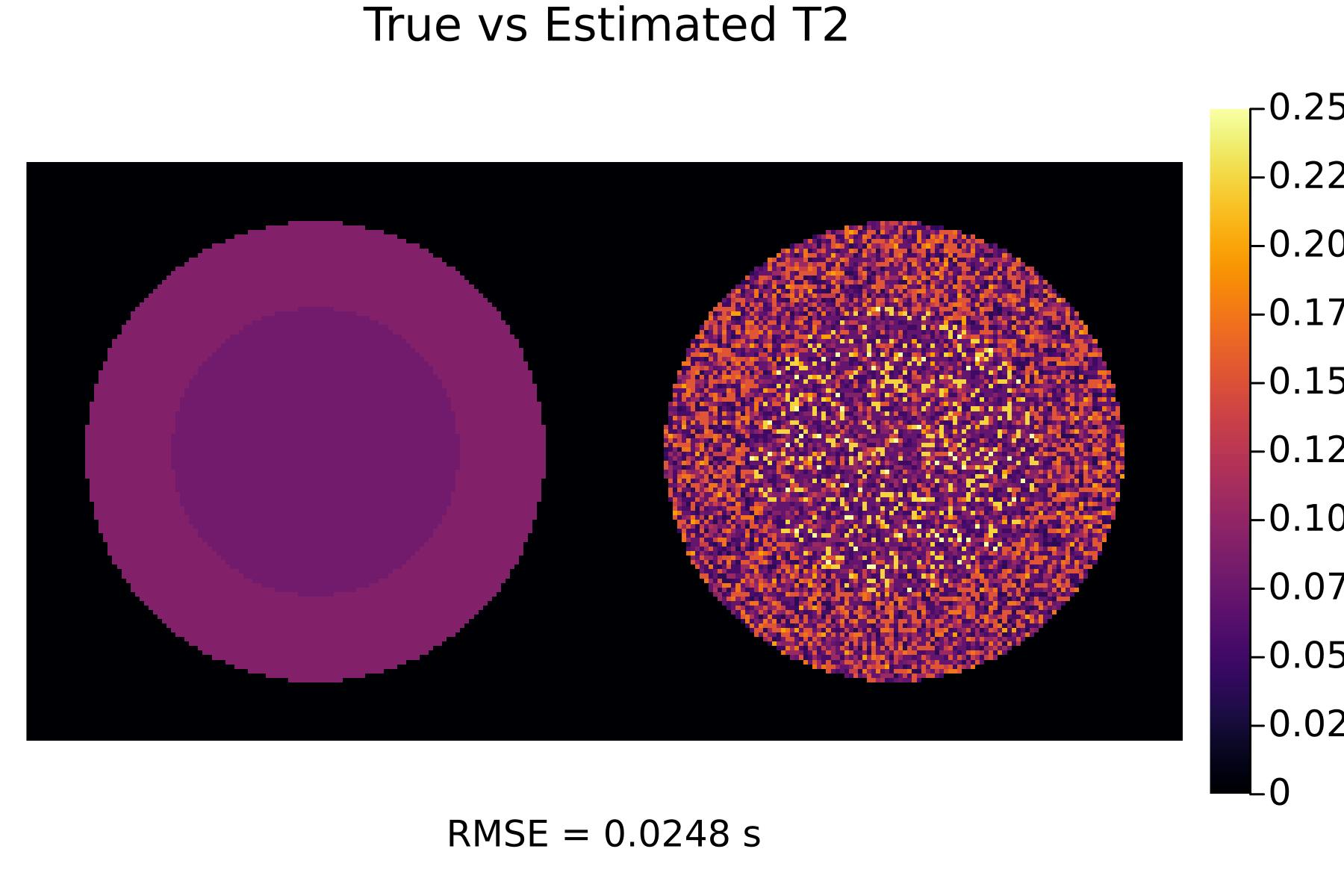
p_T2 = plot_true_vs_est(T2_true, T2_est, "True vs Estimated T2", T2_rmse, (0, 0.25))
return (p_T1, p_T2)
end
First, let's see the results with no optimization:
TR_init = [0.005, 0.005, 0.005]
flip_init = [30, 60, 80]
(p_T1_init, p_T2_init) = run(TR_init, flip_init)
display(p_T1_init)
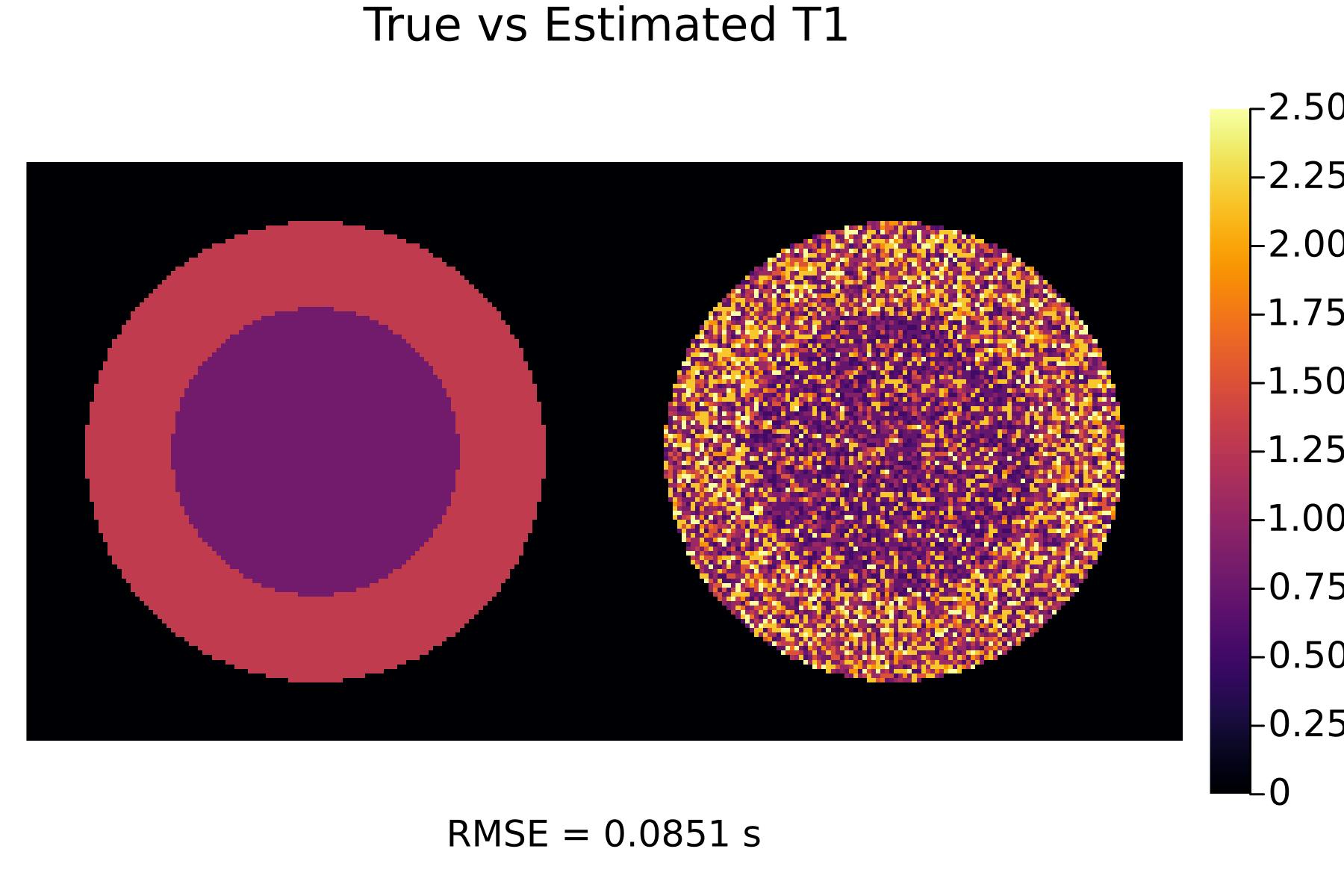
display(p_T2_init)
Now let's optimize the scan parameters and then see how the tissue parameter estimates look:
(TR_opt, flip_opt) = scan_optimization(TR_init, flip_init)
(p_T1_opt, p_T2_opt) = run(TR_opt, flip_opt)
display(p_T1_opt)
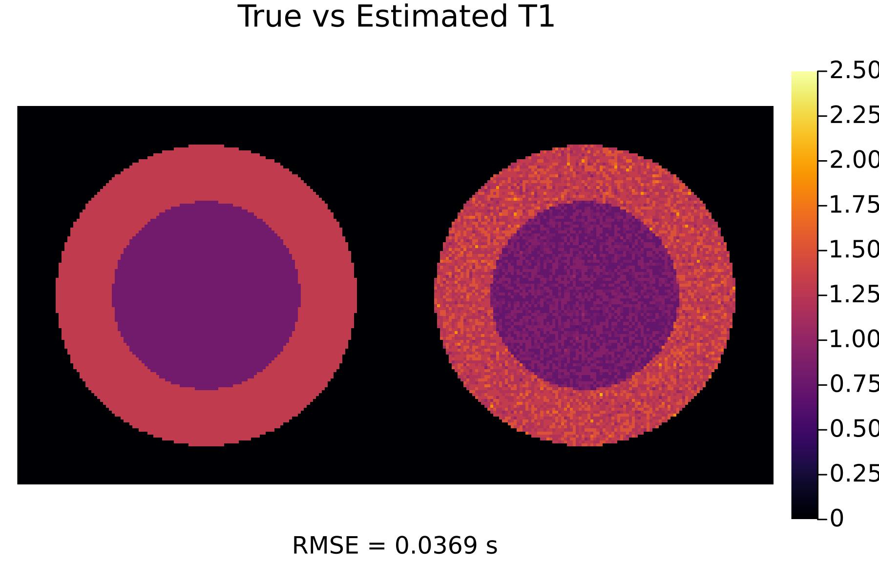
display(p_T2_opt)
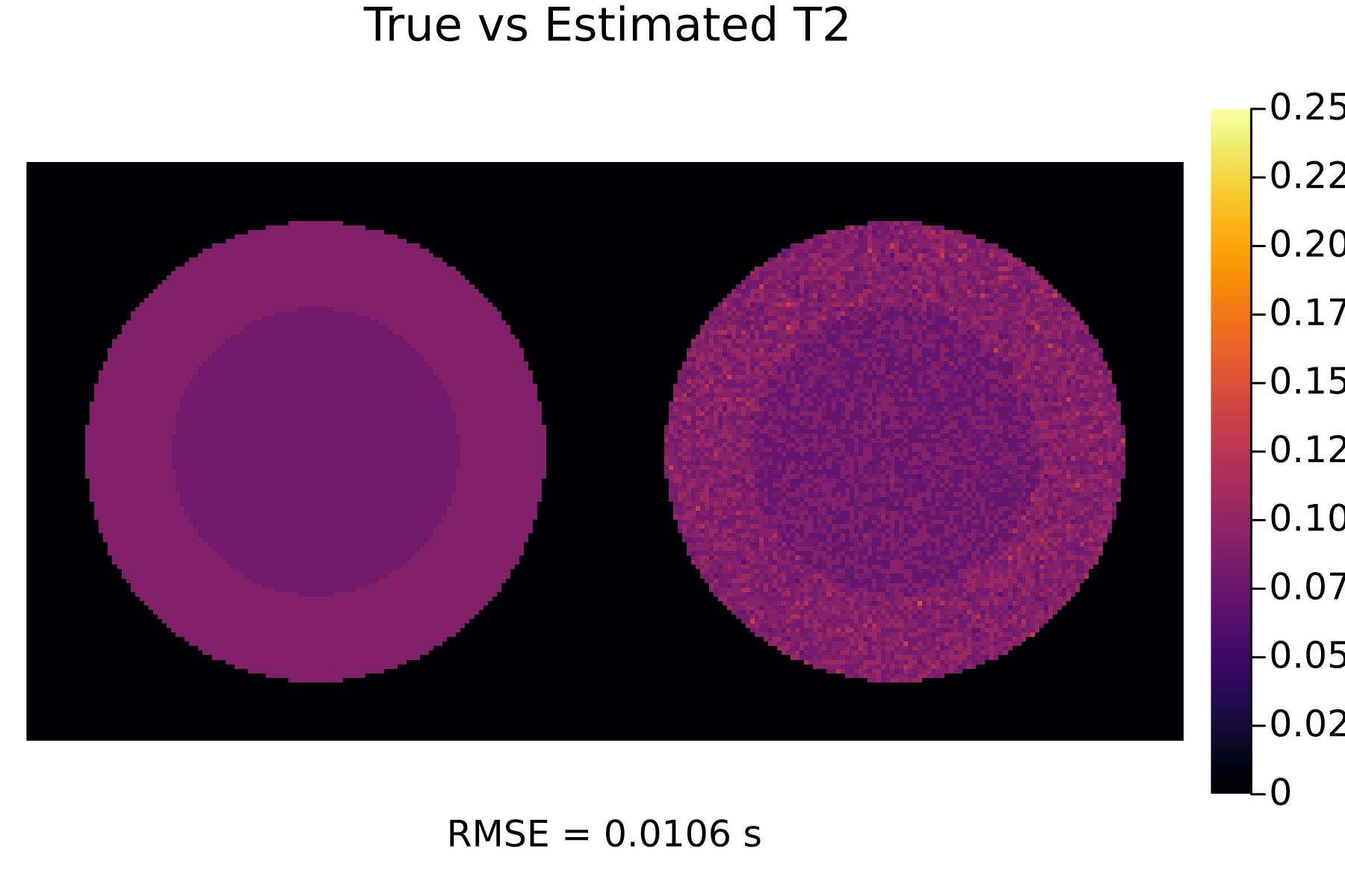
We can see that the optimized scans result in much better tissue parameter estimates!
Summary
In this post, we saw how Julia can be used to optimize MRI scan parameters to improve tissue parameter estimates. Even though we discussed MRI specifically, the concepts presented here easily extend to other applications where signal models are known and optimization is required.
Note that most of the code for this post was taken from a Dash app I helped create for JuliaHub. Feel free to check it out if you want to see this code in action!
Additional Links
- Optimizing MRI Scans Dash App
- Web app showcasing the capabilities discussed in this post.
- Optimizing MRI Scans Pluto Notebook
- Pluto notebook accompanying the Dash app mentioned above. (Unfortunately, the data used in the notebook didn't get set up properly, so most of the code can't run correctly.)
- Links to other blog posts discussing how to do MRI in Julia:
- Optimization.jl Docs
- Official documentation for Optimization.jl.